How to Create Pivot Tables in Microsoft Excel: Quick Guide

PivotTables are the closest thing Excel has to a “make my data make sense” button. You take a messy pile of rows,
wave your cursor like a tiny accountant-wizard, and suddenly you’ve got totals, trends, and tidy summarieswithout
building a Frankenstein monster of formulas.

This quick guide walks you through creating PivotTables in Microsoft Excel (desktop and Excel for the web),
then levels you up with the most useful features: sorting, filtering, grouping dates, showing percentages,
adding slicers, refreshing correctly, and avoiding the classic “Why is my PivotTable yelling (blank) at me?” moment.

What a PivotTable Is (and Why You’ll Use It Constantly)

A PivotTable is an interactive summary report. It lets you reorganize (“pivot”) the same dataset to answer different
questions fastlike revenue by region, units by product, or sales by monthwithout rewriting formulas every time your
boss says, “Cool… now do it by quarter.”

PivotTables are perfect for questions like:

• “What’s total revenue by region and by product?”
• “Which rep sold the most units last month?”
• “Show me each department’s headcount and percentage of total.”
• “Can we filter this report to only Q4 and make it clickable?”

Step 0: Prep Your Data So the PivotTable Doesn’t Panic

Most PivotTable “errors” aren’t PivotTable problemsthey’re data problems wearing a fake mustache. Before you create
your PivotTable, do a quick data tune-up.

Checklist: Your data should look like a simple table

• One header row with clear column names (no blank headers).
• No completely blank rows or columns inside the dataset.
• No merged cells in the data range (merged cells are chaos in a trench coat).
• Consistent data types (dates are real dates, numbers are real numbersnot “numbers” stored as text).
• Each column is a field (Region, Date, Product, Revenue), and each row is a record (one transaction).

Pro move: Turn your range into an Excel Table

Click anywhere in your dataset, then use Insert > Table (or Home > Format as Table).
Tables automatically expand when you add new rows and make PivotTables easier to refresh.

Step 1: Create the PivotTable (Desktop Excel)

1. Click any cell inside your dataset (or Excel Table).
2. Go to Insert > PivotTable.
3. Confirm the data range/table name.
4. Choose where to place it: New Worksheet is usually the cleanest choice.
5. Click OK.

Shortcut option: Recommended PivotTables

If you want Excel to suggest layouts, use Insert > Recommended PivotTables.
It’s like letting Excel do the first draftthen you edit it into something impressive.

Step 1 (Web Version): Create a PivotTable in Excel for the Web

1. Select the table or range.
2. Choose Insert > PivotTable.
3. Select a destination (new or existing sheet).
4. Pick a recommended layout or build your own fields.

Step 2: Build the PivotTable Using the Fields Pane

After creating the PivotTable, you’ll see the PivotTable Fields pane (sometimes called the field list).
This is your control panel. You drag fields into four areas:

• Rows: Categories listed down the left (e.g., Region, Product).
• Columns: Categories across the top (e.g., Month, Channel).
• Values: The numbers being calculated (Sum of Revenue, Count of Orders).
• Filters: Global filters for the whole report (e.g., Year = 2026).

A tiny example dataset

Imagine your data looks like this:

Example PivotTable goal: Revenue by Region

1. Drag Region to Rows.
2. Drag Revenue to Values.
3. Excel will default to Sum of Revenue (usually what you want).

Congratsyou just made a report that would otherwise take 20 minutes and three emotional support coffees.

Step 3: Change the Calculation (Sum, Count, Average, and Friends)

Sometimes Excel guesses wrong. Example: if your Revenue column contains a blank or a text value, Excel may default to
Count instead of Sum. Fix it like this:

1. In the Values area, click the dropdown next to the value field (e.g., “Sum of Revenue”).
2. Select Value Field Settings.
3. Choose Sum, Count, Average, Max, etc.
4. Click OK.

Format numbers so your PivotTable doesn’t look like it’s guessing

In Value Field Settings, click Number Format. Set Currency, Accounting,
comma style, decimals, percentageswhatever matches reality. (Your future self will say thank you.)

Step 4: Sort, Filter, and Drill Down (a.k.a. “Show Me the Receipts”)

Sorting

Click a number in the PivotTable and sort largest-to-smallest to instantly see top regions/products/reps.

Filtering

Use the dropdown arrows in Row/Column labels, or drag a field into Filters to filter the entire report.
Filtering is how PivotTables go from “summary” to “interactive dashboard energy.”

Drill down to the underlying rows

Double-click a Value cell (like West revenue) and Excel creates a new sheet with the exact source rows behind that number.
It’s one of the fastest ways to answer “Where did this total come from?”

Step 5: Group Dates (Monthly, Quarterly, Yearly) Like a Pro

If you have a Date field, you can group it so your PivotTable doesn’t list 783 individual dates like a diary.

1. Drag Date into Rows (or Columns).
2. Right-click any date in the PivotTable.
3. Select Group.
4. Choose Months, Quarters, Years (or a combo), then click OK.

If Group is grayed out

• Check for blank cells in the Date column.
• Confirm your dates are true date values (not text).
• Remove weird entries like “TBD” (PivotTables do not negotiate with “TBD”).

Step 6: Show Values As Percent of Total (Instant Insight Upgrade)

Want to know not just totals, but contribution? Use “Show Values As.”

1. Click a value in the PivotTable.
2. Right-click > Show Values As.
3. Pick % of Grand Total, % of Column Total, Running Total In,
   or % Difference From.

Trick: Show both dollars and percent

Drag the same numeric field into Values twice (e.g., Revenue appears two times).
Set the second one to “% of Grand Total.” Now you’ve got a scoreboard and the percentage breakdown side-by-side.

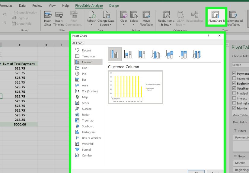
Step 7: Add Slicers and Timelines (So People Can Click Things)

Slicers are big, friendly filter buttons. Timelines are slicers for dates. They’re perfect when you’re building a
report for other humans (instead of spreadsheet monks).

Insert a Slicer

1. Click inside the PivotTable.
2. Go to PivotTable Analyze (or Options depending on your version).
3. Select Insert Slicer.
4. Choose fields like Region, Product, Rep, then click OK.

Insert a Timeline

1. Click inside the PivotTable.
2. Select Insert Timeline.
3. Choose your Date field.
4. Filter by Year/Quarter/Month/Day using the timeline controls.

Step 8: Refresh Your PivotTable (Because Data Changes… Rudely)

If your PivotTable isn’t updating after you add new rows, don’t rebuild itrefresh it.

• Refresh: Click the PivotTable > PivotTable Analyze > Refresh.
• Refresh All: Refreshes all PivotTables and connections in the workbook.

Why it still won’t refresh correctly

• Your PivotTable range doesn’t include new rows (Excel Tables fix this).
• New data has mismatched headers or blank headers.
• Numbers are stored as text, so sums behave strangely.

Step 9: Common PivotTable Problems (and Quick Fixes)

Problem: “(blank)” shows up everywhere

• Fix the source data: fill missing values or label them (e.g., “Unknown”).
• Filter out (blank) in the PivotTable field dropdown.

Problem: Totals look wrong

• Check the calculation (Sum vs Count).
• Confirm numeric fields are truly numbers.
• Watch for duplicates in source data (PivotTables summarize what you give themgood or bad).

Problem: PivotTable layout looks messy

• Use Design tab: Report Layout (Compact/Outline/Tabular).
• Turn off repeating subtotals if they’re cluttering the view.
• Apply a PivotTable style for instant readability.

Step 10: Two “Advanced” Features That Are Worth Learning Early

Calculated Fields (basic custom math)

If you need a simple formula inside the PivotTable (like Revenue per Unit), you can add a calculated field.
This is handy for basic ratios, but for more complex modeling (especially across multiple tables), Excel’s Data Model
tools are often a better fit.

Multiple Tables and Relationships (Data Model)

If your analysis needs more than one tablelike Sales + Products + RegionsExcel can build relationships so your
PivotTable can pull fields across tables without manually VLOOKUP-ing everything into one mega-sheet.
This is powerful, but not every Excel platform supports every feature the same way.

Quick “Do This, Not That” PivotTable Cheatsheet

• Do: Use an Excel Table as the data source. Not: A mystery range that never expands.
• Do: Name your headers clearly. Not: Leave blank columns and hope for the best.
• Do: Format values via Value Field Settings. Not: Format random cells and pray it sticks.
• Do: Add the same value twice for $ + %. Not: Build a separate report for percentages.
• Do: Refresh after updates. Not: Rebuild the whole PivotTable every Tuesday.

Common Real-World Experiences (500+ Words): What Actually Happens When You Use PivotTables

Let’s talk about the part no one mentions in neat tutorials: PivotTables are amazing in the real world because real
world data is… not amazing. The “experience” of working with PivotTables usually falls into three stages:
(1) instant victory, (2) mild confusion, (3) unstoppable competence (with occasional dramatic sighs).

Stage 1 is the honeymoon. You build your first PivotTable, drag Region into Rows, Revenue into Values, and suddenly
you’ve got totals that look like you spent the afternoon doing careful math instead of clicking two things.
This is where people say, “Wait… that’s it?” Yes. That’s it. PivotTables are basically Excel’s reward for keeping
your data in columns like a responsible adult.

Stage 2 is where the “fun” begins. Someone adds new rows to the dataset, and your PivotTable doesn’t change.
You refresh. Still weird. You refresh again (because surely Excel just didn’t hear you the first time).
The real fix is usually one of these: your source range didn’t include the new rows, your headers shifted, or the new
data introduced a sneaky typolike “West ” (with a trailing space) becoming a whole new region. This is why using an
Excel Table as the source feels like unlocking a secret door: it expands automatically, and refresh suddenly works the
way your optimism thinks it should.

Another very common moment: you try to group dates and Excel refuses. The Group option is grayed out like it’s
emotionally unavailable. The cause is almost always “Date” values that aren’t real datesmaybe they were imported
from a system that stored them as text, or there are blanks, or one row says “N/A.” Once you clean that column
(convert to dates, remove blanks, replace weird values), grouping becomes your best friend. Grouping is what turns a
daily transaction log into a monthly trend report in seconds, which is the difference between “interesting” and
“executive-ready.”

Then there’s the classic “(blank)” invasion. PivotTables are honestpainfully honest. If your source data has missing
Region values, the PivotTable will absolutely show you a bucket called (blank), like a spotlight on your data hygiene.
In practice, most teams either fill those blanks upstream (best), label them “Unknown” (good), or filter them out
(acceptable if you’re sure they shouldn’t count). The key experience here is learning that PivotTables don’t create
problems; they reveal them. Like a very polite mirror.

Finally, once you’ve built a few PivotTables, you start using “Show Values As” constantly. It’s one thing to know
revenue totals; it’s another to see that the West is 42% of total revenue while the East is 18%. That’s the moment
PivotTables stop being a reporting tool and start being an analysis tool. Add slicers and timelines, and suddenly
your report becomes something a manager can explore without calling you every five minutes. The best real-world
PivotTable experience is when your inbox gets quieter because the dashboard answers the questions before they’re asked.

Conclusion

Creating PivotTables in Microsoft Excel is mostly about two things: clean source data and confident field placement.
Start with a tidy table, create the PivotTable from the Insert tab, drag fields into Rows/Columns/Values, then level
up with grouping, Show Values As, slicers, and refresh discipline. Do that, and PivotTables become less of a “feature”
and more of a superpowerminus the cape, plus the credibility.